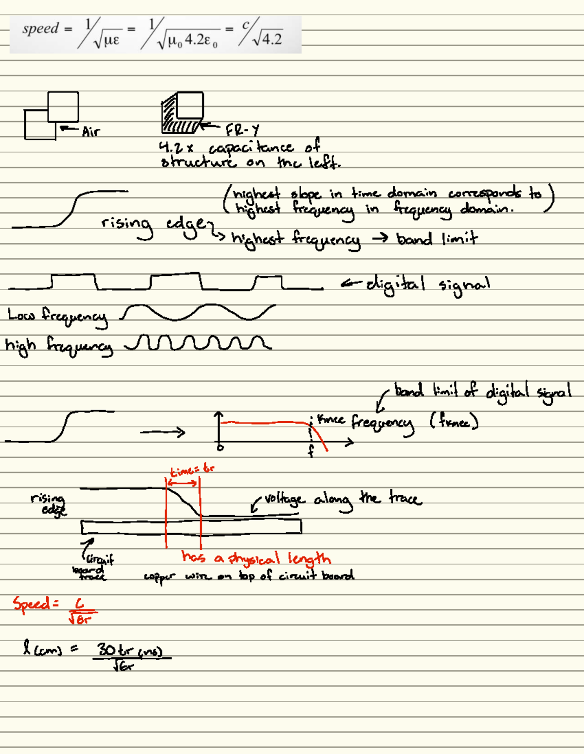
Rising times represent a fundamental temporal and physical measurement across various technical fields, denoting the duration required for a system, signal, or celestial body to transition from a lower baseline state to a specified upper threshold. Whether applied in electronics to evaluate waveform propagation, in meteorology to track atmospheric phenomena, or in astronomy to calculate stellar and lunar elevations, mastering this metric is essential for precise analysis, system optimization, and accurate forecasting.
Defining Rising Times Across Technical Disciplines
The concept of a rising time is not monolithic; its definition, calculation, and practical implications change significantly depending on the industry and the physical phenomena being observed. At its core, the metric always concerns a transition from an initial reference point to a final operational state over a measured duration, but the physical laws and instrumentation governing that transition vary widely.
In electrical engineering and electronics, rising time typically quantifies how rapidly a signal transitions from a low voltage state to a high voltage state. In astronomy, it refers to the precise moment a celestial body crosses the eastern horizon, influenced by geographic coordinates and axial tilt. Understanding these disciplinary nuances prevents conceptual confusion and ensures that technical specifications are interpreted correctly within their intended context.
To appreciate the scope of rising times, professionals must look past simple definitions and examine the underlying mathematical models and hardware limitations that dictate these durations. The following sections break down how different industries measure, analyze, and optimize rising times to achieve desired operational outcomes.
Rising Times in Electronics and Signal Processing
In digital and analog electronics, the rising time of a pulse or waveform is universally defined as the time interval required for the signal amplitude to change from a specified low value to a specified high value. By convention in most engineering applications, these thresholds are set at 10% and 90% of the step height, bypassing the non-linear asymptotic tails at the very beginning and end of the transition.
The Mathematics of Signal Transition
The speed at which a circuit can switch states dictates the maximum clock frequency and data throughput of digital systems. When a voltage step is applied to a reactive network containing resistance, capacitance, and inductance (RC or RLC circuits), the output waveform does not change instantaneously. Instead, it follows an exponential charging curve governed by the time constant $\tau = RC$.
The output voltage $V(t)$ as a function of time during a step response is expressed as:
$$V(t) = V_{max} \left(1 - e^{-\frac{t}{\tau}}\right)$$
To calculate the 10% to 90% rising time ($t_r$), engineers solve for the time difference between $0.1 V_{max}$ and $0.9 V_{max}$:
$$t_r \approx 2.2 \times \tau$$
This relationship highlights that reducing parasitic capacitance or source resistance is the primary method for shortening rising times and increasing circuit speed.
Practical Implications for High-Speed Design
As data rates climb into the gigahertz range, managing rising times becomes critical for signal integrity. Extremely fast rising times—often desired for low propagation delay—introduce high-frequency harmonic components that can cause electromagnetic interference (EMI), ringing, and signal reflection on improperly terminated transmission lines. Conversely, excessively slow rising times can lead to logic ambiguity, increased power dissipation in CMOS gates during the transition phase, and timing violations in synchronous digital logic.
| Field / Application | Standard Thresholds | Primary Determining Factor | Common Engineering Challenge |
|---|---|---|---|
| Digital Logic (CMOS) | 10% to 90% of $V_{DD}$ | Gate capacitance and load resistance | Minimizing propagation delay without causing ringing |
| Oscilloscope Probes | 10% to 90% of step amplitude | Bandwidth ($BW \times t_r \approx 0.35$) | Ensuring probe bandwidth exceeds signal harmonics |
| Power Electronics | 10% to 90% or 5% to 95% | Gate charge ($Q_g$) of MOSFET/IGBT | Balancing switching losses with electromagnetic interference |
| Astronomy / Ephemeris | Horizon to Zenith / Meridian | Latitude, declination, and refraction | Accounting for atmospheric bending at low elevations |
Rising Times in Astronomy and Celestial Mechanics
In observational astronomy, rising time refers to the precise local sidereal or standard time at which the upper limb of a celestial body—such as the Sun, Moon, planets, or stars—appears on the eastern horizon. Unlike electronic square waves, astronomical rising times are governed by celestial mechanics, Earth's rotational dynamics, and the observer's geographic position.
Calculating Celestial Rising and Setting
The calculation of a celestial body's rising time involves spherical trigonometry. The local hour angle ($H$) of the body when it is on the horizon can be determined using the observer's geographic latitude ($\phi$) and the body's declination ($\delta$):
$$\cos(H) = -\tan(\phi) \times \tan(\delta)$$
Once the hour angle is converted into time units, it is combined with the body's right ascension and the local sidereal time to yield the exact clock time of the rising event. However, theoretical calculations must be adjusted for physical real-world factors.
Environmental and Atmospheric Adjustments
Two primary atmospheric phenomena alter the observed rising times of celestial objects compared to their calculated geometric positions:
- Atmospheric Refraction: Earth's atmosphere bends light rays coming from space, making celestial bodies appear higher above the horizon than they actually are. Because of this refraction—which accounts for approximately 34 arcminutes at the horizon—a star or the Sun appears to rise slightly earlier than geometric calculations predict.
- Semidiameter and Parallax: For extended bodies like the Sun and the Moon, the standard astronomical convention defines rising time as the moment the upper limb touches the horizon, rather than the center of the disk. This adds a correction factor based on the angular radius of the object and, in the case of the Moon, its parallax distance from the Earth.
Comparative Analysis of Rising Time Metrics
To better understand how rising times function across different technical domains, it is helpful to compare their operational parameters, measurement tools, and core objectives side by side.
| Feature / Domain | Electronics & Signal Processing | Astronomy & Geodesy | Physiology & Exercise Science |
|---|---|---|---|
| Primary Medium | Voltage, current, or optical photons | Celestial coordinates and horizons | Heart rate, blood pressure, or muscle tension |
| Standard Measurement Unit | Nanoseconds (ns) or picoseconds (ps) | Hours, minutes, UTC / Local Time | Seconds (s) or minutes (min) |
| Key Instrumentation | Digital storage oscilloscopes, TDRs | Ephemeris tables, astrolabes, GPS sensors | Electrocardiograms (ECG), sphygmomanometers |
| Optimization Goal | Maximizing speed while limiting EMI | Accurate scheduling for observation and navigation | Assessing cardiovascular recovery and autonomic function |
Measuring and Verifying Rising Times
Accurate measurement of rising times requires specialized instrumentation and strict adherence to calibration protocols. In electronic testing, engineers rely on high-bandwidth oscilloscopes paired with active probes to capture fast transients without distorting the waveform.
Step-by-Step Measurement Procedure in Electronics
- Connect the Probe: Attach a low-capacitance active probe or a matched passive probe to the test point, ensuring the ground loop is kept as short as possible to prevent inductive ringing.
- Set Bandwidth Limits: Configure the oscilloscope bandwidth limit to match the expected frequency content of the signal, reducing high-frequency noise that can distort the 10% and 90% threshold measurements.
- Trigger and Acquire: Establish a stable edge trigger on the rising edge of the pulse. Acquire multiple waveform averages to eliminate random jitter.
- Apply Cursors or Automatic Measurements: Enable the oscilloscope's automated rise time measurement function. If measuring manually, place vertical cursors at the intersection of the waveform with the 10% and 90% amplitude graticules.
- Calculate Bandwidth Correction: If the rising time of the signal is close to the rising time of the oscilloscope itself, apply the root-sum-square correction formula: $$t_{r,\text{actual}} = \sqrt{t_{r,\text{measured}}^2 - t_{r,\text{scope}}^2}$$
Common Challenges and Troubleshooting
When rising times do not conform to theoretical expectations or system design specifications, engineers and technicians must systematically isolate the root cause.
Slow Rising Times in Digital Circuits
- Excessive Capacitive Load: High fan-out or long trace lengths increase load capacitance ($C_L$), lengthening the RC time constant. Solution: Buffer the signal or reduce trace length.
- Weak Driver Strength: The output impedance ($R_o$) of the driving logic gate is too high. Solution: Select a driver with lower output resistance or parallel multiple gates.
Jitter and Instability in Waveform Edges
- Power Supply Noise: Voltage droop on the VCC rail during switching events alters the threshold crossing points. Solution: Add decoupling capacitors close to the IC power pins.
- Improper Termination: Unmatched transmission line impedance causes reflections that distort the rising edge. Solution: Implement series source termination or parallel load termination.
Frequently Asked Questions
Why is rising time measured from 10% to 90% instead of 0% to 100%?
Real-world waveforms rarely transition along a clean, sharp mathematical line. The bottom 0% to 10% and top 90% to 100% segments often feature non-linear rounding, asymptotic tails, and noise jitter that make accurate manual or automated start/stop identification unreliable. The 10% to 90% window captures the steepest, most linear portion of the transition curve consistently.
How does oscilloscope bandwidth affect rising time measurements?
An oscilloscope has its own internal rising time determined by its analog bandwidth ($BW$). If an oscilloscope has a bandwidth of 100 MHz, its native rise time is approximately $0.35 / 100\text{ MHz} = 3.5\text{ ns}$. If you attempt to measure a signal with a 3.5 ns rise time using this scope, the measured result will be artificially slowed because the instrument's response time is factored into the reading.
Can rising times be too fast in circuit design?
Yes. While high-speed digital systems require fast rising times for high data throughput, excessively fast edges contain high-frequency harmonic energy that exacerbates electromagnetic interference (EMI), creates severe ground bounce, and causes signal overshoot and ringing on unterminated transmission lines.
What is the relationship between rising time and frequency response?
In linear systems, there is an inverse relationship between the upper cutoff frequency ($f_c$) and the pulse rise time ($t_r$). This is commonly approximated by the product rule $t_r \times f_c \approx 0.35$ for a single-pole system. A wider bandwidth allows for faster rising times and more faithful reproduction of high-frequency signal details.
How do atmospheric conditions alter astronomical rising times?
Earth's atmosphere refracts light, bending the rays of celestial bodies downward toward the horizon. This optical bending makes objects appear to rise several minutes earlier than they would on an airless planet like the Moon. Temperature and barometric pressure fluctuations can cause minor variations in this refraction index.
Conclusion and Next Actions
Mastering the concept and measurement of rising times requires a firm grasp of both theoretical mathematics and practical instrumentation limits. Whether designing high-speed printed circuit boards, scheduling astronomical observations, or analyzing dynamic physical systems, always verify your baseline thresholds and ensure your measurement tools possess adequate bandwidth. Begin by auditing your current signal paths or ephemeris calculation models to identify any sources of latency, jitter, or calibration error.