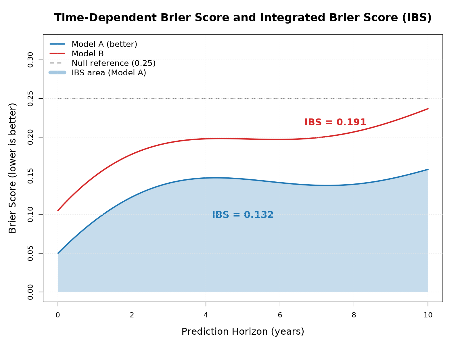
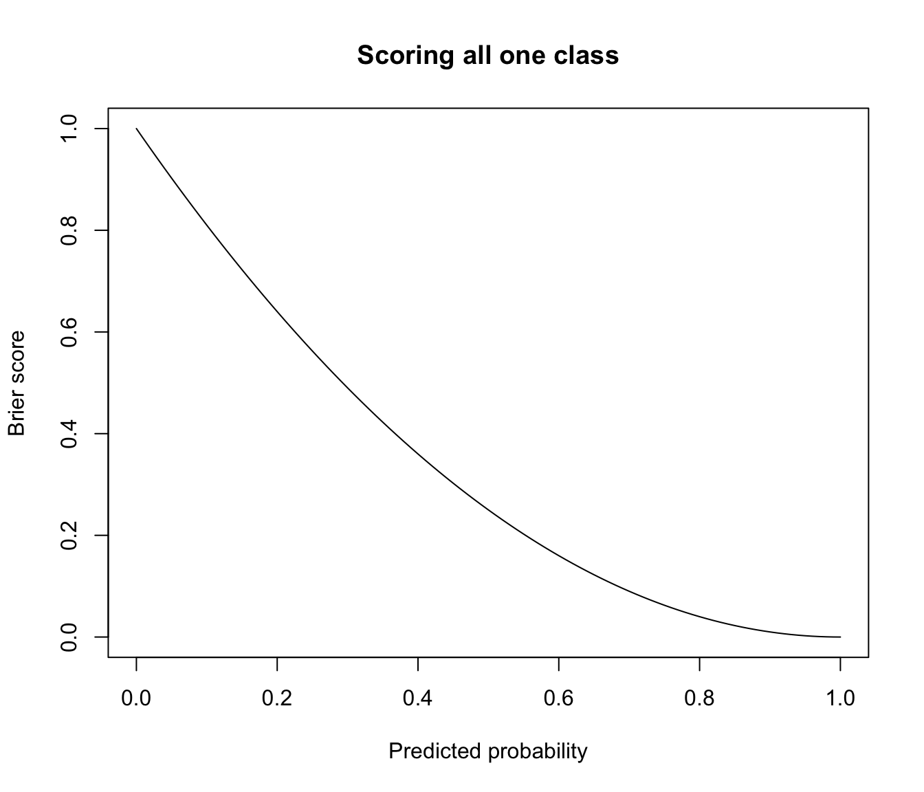
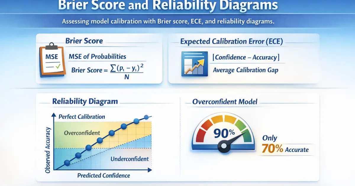
A Brier score is a metric used to measure the accuracy of probabilistic predictions by calculating the mean squared difference between predicted probabilities and the actual binary outcomes that occur. Ranging from 0.0 to 1.0, a lower score indicates higher forecast accuracy, making it an essential tool in meteorology, finance, and machine learning.
Understanding the Fundamentals of Probability Forecasts
Traditional forecasting often relies on categorical statements, such as "it will rain tomorrow" or "the stock price will rise." While intuitive, these binary declarations fail to capture the inherent uncertainty of complex systems. Probabilistic forecasting addresses this limitation by assigning a numerical likelihood—expressed as a percentage or decimal between 0 and 1—to a potential future event. For example, stating there is a 70% chance of precipitation acknowledges nuance while providing actionable risk data.
However, introducing probabilistic estimates creates a verification challenge. If a meteorologist predicts a 70% chance of rain and it does not rain, was the forecast wrong? Not necessarily, as a 30% chance of non-occurrence remains viable. Evaluating these types of predictions requires a specialized scoring rule that rewards both accuracy and calibration. Calibration measures how closely predicted probabilities align with long-term empirical frequencies, ensuring that when an event is predicted to happen 70% of the time, it actually occurs roughly 70% of the time.
To handle these requirements, forecasters and data scientists rely on strictly proper scoring rules. A scoring rule is "proper" if forecasters maximize their expected score by reporting their true subjective beliefs rather than hedging. The Brier score is one of the most prominent proper scoring rules used for binary and categorical events. It bridges the gap between raw probability estimates and tangible outcomes, giving modelers an objective baseline for performance improvement.
The Mathematical Foundation of the Brier Score
Introduced by meteorologist Glenn W. Brier in 1950, the Brier score is fundamentally the mean squared error of probability forecasts. For a set of $N$ predictions, the standard formula for a binary outcome is:
$$BS = \frac{1}{N} \sum_{i=1}^{N} (f_i - o_i)^2$$
In this equation:
- $f_i$ represents the forecasted probability of the event occurring for observation $i$, expressed as a value between 0 and 1.
- $o_i$ represents the actual observed outcome for observation $i$, taking a value of 1 if the event occurred and 0 if it did not.
- $N$ is the total number of forecasts evaluated.
To understand how this operates in practice, consider a simple manual calculation. Suppose a weather service issues five forecasts for a specific rain event, and we track whether rain actually occurred:
| Observation ($i$) | Forecast Probability ($f_i$) | Actual Outcome ($o_i$) | Difference ($f_i - o_i$) | Squared Error $(f_i - o_i)^2$ |
|---|---|---|---|---|
| 1 | 0.80 | 1 | -0.20 | 0.0400 |
| 2 | 0.20 | 0 | 0.20 | 0.0400 |
| 3 | 0.90 | 1 | -0.10 | 0.0100 |
| 4 | 0.40 | 1 | -0.60 | 0.3600 |
| 5 | 0.10 | 0 | 0.10 | 0.0100 |
Summing the squared errors yields $0.04 + 0.04 + 0.01 + 0.36 + 0.01 = 0.46$. Dividing by the number of observations ($N = 5$) results in a Brier score of $0.46 / 5 = 0.092$.
Because it is a squared error metric, the Brier score heavily penalizes confident, incorrect predictions. If a model predicts a 0.99 probability of an event occurring, but the event fails to materialize ($o_i = 0$), the squared error contribution is $(0.99 - 0)^2 = 0.9801$. This severe penalty encourages models to remain well-calibrated and discourages unjustified overconfidence.
Interpreting Brier Scores and Benchmarks
Interpreting a Brier score requires understanding its scale and baseline reference points. The score ranges from 0.0 to 1.0 for binary events:
- 0.0: Represents a perfect set of forecasts where every occurrence was assigned a 100% probability and every non-occurrence a 0% probability.
- 1.0: Represents completely inaccurate forecasts where every occurrence was assigned a 0% probability and every non-occurrence a 100% probability.
A common point of confusion for beginners is establishing what constitutes a "good" Brier score. Unlike accuracy percentages, where 95% is universally strong, Brier scores depend heavily on the base rate (climatology) of the event being predicted. For rare events, achieving a low Brier score is deceptively simple by always predicting zero, yet that trivial model holds no practical value.
To illustrate this, consider predicting a rare medical condition that affects only 2% of a population ($o = 0.02$). A naive model that blindly guesses a 2% probability for every patient will yield a very low Brier score, even though it provides zero diagnostic utility. Therefore, analysts often decompose the Brier score or compare it against a reference climatological forecast using the Brier Skill Score (BSS):
$$BSS = 1 - \frac{BS}{BS_{ref}}$$
Where $BS$ is the model's Brier score and $BS_{ref}$ is the Brier score of a reference forecast, such as historical sample averages. A positive BSS indicates that the model outperforms the reference baseline, while a negative score indicates the model is worse than a naive historical guess.
Decomposition of the Brier Score
To gain deeper diagnostic insights into model performance, the standard Brier score can be mathematically decomposed into three distinct components: Uncertainty, Reliability, and Resolution. First formulated by Allan H. Murphy in 1973, this decomposition reveals why a model received a particular score.
1. Uncertainty
Uncertainty measures the inherent variability of the observed outcomes. It depends solely on the sample climatology (the base rate of the event) and represents the baseline difficulty of the forecasting task. A rare event or an event split evenly 50/50 has a fixed uncertainty value that cannot be altered by a forecasting system. It serves as the irreducible floor of predictability for that specific dataset.
2. Reliability (Bias)
Reliability measures how closely the predicted probabilities correspond to the actual empirical frequencies. For example, if a model groups all predictions into bins around 30% and the event actually occurs 30% of the time within those instances, the reliability component is zero, indicating excellent calibration. High reliability means the model's confidence levels match reality.
3. Resolution
Resolution measures the model's ability to categorize events into distinct subsets that diverge from the overall climatological sample average. A model with good resolution issues forecasts that vary widely based on incoming data—assigning high probabilities when events happen and low probabilities when they do not—rather than defaulting to safe, middle-of-the-road probabilities like 50% for every scenario.
By analyzing these three components, data scientists can diagnose model flaws. A model might be highly uncertain due to noisy data, yet possess great resolution; conversely, a model might be consistently biased, showing poor reliability that requires recalibration via techniques like Platt scaling or isotonic regression.
Applications Across Industries
While originally developed for weather forecasting, the Brier score has become a vital metric across several data-intensive industries where probabilistic validation is paramount.
Meteorology and Climate Science
Weather forecasting remains the primary domain for Brier scores. Modern numerical weather prediction (NWP) systems utilize ensemble forecasting—running multiple simulations with slightly perturbed initial conditions—to generate probability distributions for precipitation, temperature thresholds, and severe storm tracks. Meteorological agencies use Brier scores to continuously audit model performance, compare competing atmospheric models, and track improvements in forecasting skill over decades.
Machine Learning and Classification
In machine learning, binary classification models such as logistic regression, random forests, and gradient boosting output probabilities rather than hard class labels (e.g., predicting the probability that a customer will churn or that a transaction is fraudulent). While metrics like Area Under the Receiver Operating Characteristic Curve (ROC-AUC) measure ranking ability, the Brier score evaluates calibration. A model can have a high ROC-AUC yet suffer from poor probability calibration, making the Brier score an indispensable companion metric for production machine learning validation.
Finance and Risk Management
Financial institutions use probabilistic forecasting to model credit defaults, market volatility, and macroeconomic stress tests. When a bank assigns a default probability to a corporate loan portfolio, verifying those predictions against actual defaults using a Brier score ensures that capital reserve requirements align with empirical risk, satisfying regulatory frameworks such as Basel III guidelines.
Limitations and Practical Considerations
Despite its mathematical elegance and widespread adoption, the Brier score has specific limitations that practitioners must account for during evaluation.
Sensitivity to Event Base Rates
As noted earlier, the Brier score is heavily influenced by the base rate of the target event. For rare events (often called the class imbalance problem in machine learning), the baseline score can be deceptively low. A model that predicts a flat zero for a rare disease will achieve a Brier score equal to the variance of the base rate, rendering the raw number difficult to interpret without comparison to a null model.
Multi-Category Extensions
The standard Brier score applies strictly to binary outcomes. While it can be extended to multi-class classification problems through the multi-category Brier score:
$$BS_{multi} = \frac{1}{N} \sum_{i=1}^{N} \sum_{k=1}^{K} (f_{ik} - o_{ik})^2$$
where $K$ is the number of discrete classes, the interpretation grows more complex. As the number of categories increases, the squared differences across all classes must sum appropriately, requiring careful normalization to ensure fair comparisons across datasets with differing numbers of classes.
Alternative Metrics Comparison
To ensure robust validation, practitioners rarely rely on the Brier score in isolation. It is frequently compared against or combined with other scoring metrics:
- Log Loss (Cross-Entropy Loss): Unlike the Brier score, which is bounded between 0 and 1, Log Loss penalizes confident, wrong predictions infinitely. Log loss is strictly proper and often preferred in neural network training, though it can be overly sensitive to outlier predictions.
- ROC-AUC: Evaluates the model's ability to discriminate between classes across all possible classification thresholds, but ignores calibration entirely.
Best Practices for Calculating and Reporting Brier Scores
When implementing Brier score evaluations in research papers, data science pipelines, or meteorological assessments, adhering to standardized best practices ensures transparency and reproducibility.
- Establish a Climatological Baseline: Always calculate and report the Brier Skill Score alongside the raw Brier score. Contextualizing performance against a historical or naive baseline prevents misinterpretation of rare-event datasets.
- Check Probability Calibration: Before computing the final score, plot reliability diagrams (calibration curves) to visualize whether your predicted probabilities match observed frequencies visually as well as numerically.
- Handle Missing Data Consistently: Ensure that the sample size ($N$) remains identical when comparing competing models. Dropping missing observations inconsistently across model evaluations will distort comparative Brier scores.
- Use Proper Software Libraries: Implement calculations using well-tested statistical packages (such as
scikit-learnin Python viabrier_score_loss) to avoid implementation errors in manual summation loops.
Frequently Asked Questions
What is a good Brier score?
A good Brier score depends entirely on the base rate of the event being predicted. For common events with a 50% base rate, a score below 0.15 typically indicates a strong model. For rare events occurring only 1% of the time, a naive model can achieve a score of 0.01 by simply guessing zero, meaning a "good" score must be evaluated relative to a climatological baseline using the Brier Skill Score.
How does the Brier score differ from Log Loss?
The Brier score measures the mean squared error of probability predictions, bounded strictly between 0 and 1. Log Loss (cross-entropy) penalizes confident, incorrect predictions exponentially, approaching infinity as a prediction approaches 100 certainty for the wrong outcome. While Brier scores tolerate moderate overconfidence better, Log Loss penalizes it severely, making Log Loss more common in neural network optimization.
Can Brier scores be used for multi-class predictions?
Yes. The multi-category Brier score expands the formula by summing the squared differences across all possible discrete classes for each observation. This allows forecasters to evaluate probability distributions across more than two outcomes, such as predicting whether tomorrow's weather will be sunny, rainy, or snowy.
Why does a lower Brier score mean better accuracy?
Because the Brier score calculates squared errors, it measures the distance between the forecast probability and the actual binary outcome (0 or 1). Perfect predictions yield an error of zero. As errors increase, the squared value grows, meaning higher scores reflect worse predictive performance.
Is the Brier score a proper scoring rule?
Yes, the Brier score is classified as a strictly proper scoring rule. This mathematical property ensures that forecasters and machine learning models achieve their optimal expected score only by reporting their true, unhedged beliefs about the likelihood of an event.
Conclusion
The Brier score remains an indispensable metric for verifying probabilistic forecasts across meteorology, machine learning, and risk management. By measuring both accuracy and calibration through mean squared error, it penalizes unwarranted overconfidence while rewarding models that capture true uncertainty. Understanding its mathematical formulation, decomposition components, and baseline dependencies empowers analysts to evaluate models rigorously and improve decision-making under uncertainty.